Every utility-scale layout starts as a clean 2D grid. Pile columns spaced 2.65 m apart, every bay identical, every row parallel. Then the site has a slope, and the grid stops being true.
On a 13° slope, each 2.65 m bay measures 2.58 m on the ground: 7 cm short. Stake a six-pile row from the plan dimension and the last pile lands 35 cm from where the design says it should be. The same angle also drops each pile 0.60 m below its neighbor. One angle, two errors, every row.
This study walks through a real sloped site in PVX.Cad, from slope analysis to the exported pile schedule, and shows why the number the field crew needs is never the plan dimension. It is the verified X-Y-Z coordinate of every pile.
The reference geometry
The transformation needs a defined starting point. The rack is fixed-tilt at 25° module inclination, carried by 6 pile columns. Pile spacing along the rack plane is 2.65 m, the pile profile is C-Channel, bottom clearance is 0.60 m, and embedment depth is 1.50 m. These values are the nominal reference everything else is measured against.
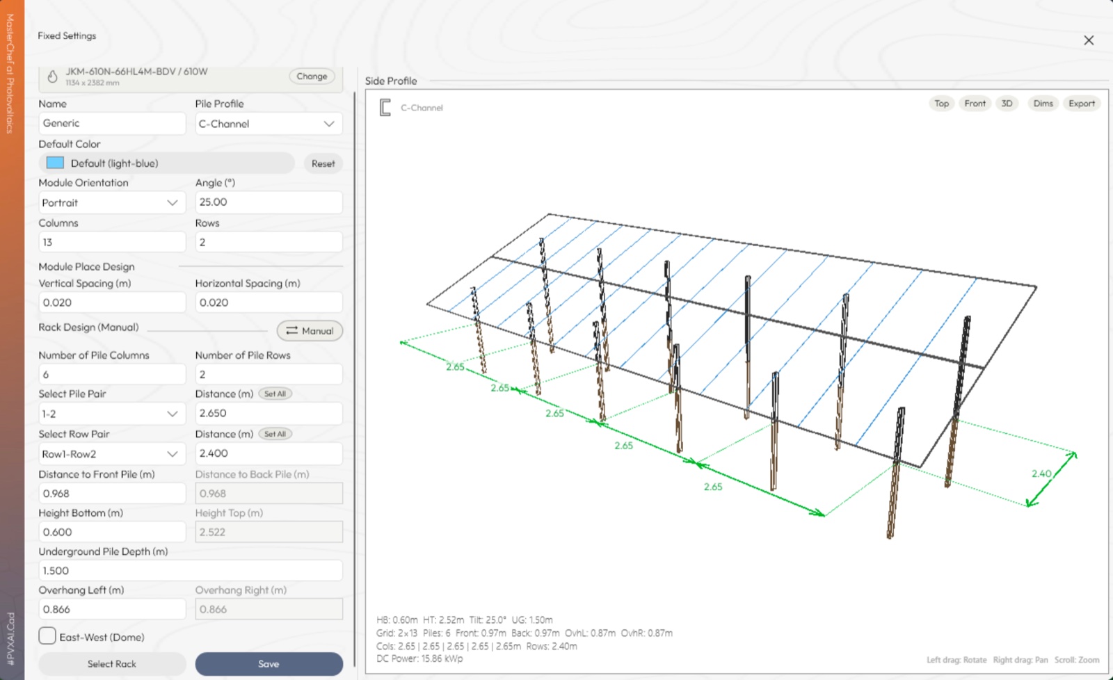
The reference rack geometry and pile parameters, defined in PVX.Cad.
In the 2D plan view, this geometry produces the grid every designer knows. Each gap reads 2.65 m. Perfectly uniform, perfectly rectangular.
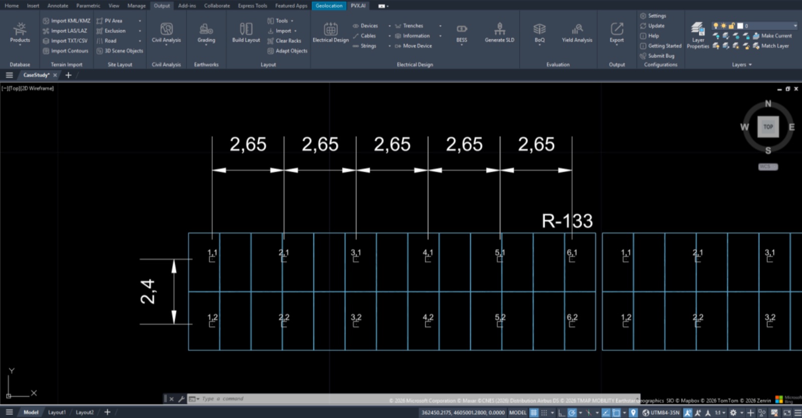
The nominal 2D plan. Every bay reads 2.65 m. This is the dimension a field crew would love to stake with. On this site, it would put piles in the wrong place.
What the slope analysis says
The first step is measuring what the terrain actually does. Slope analysis on the imported KML zone maps the gradient distribution across the site: green for gentle terrain, red for steep.
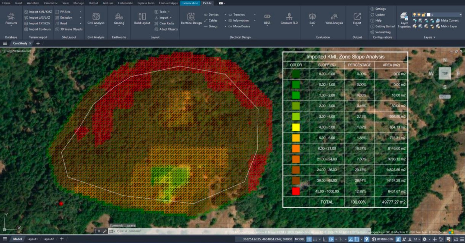
Slope analysis and distribution table for the imported site boundary.
A significant share of the site sits above 6° of slope. Localized zones reach the 36 to 45% band. The distribution is heterogeneous, which means every pile row crosses a different gradient. The horizontal projection of the pile spacing will not be one corrected number. It will vary across the site, rack by rack.
Placing the nominal grid on real terrain
With 3D terrain enabled (slope checking), the layout leaves the flat drawing plane and sits on the actual topography. Every rack and every pile is now evaluated at the real gradient of its own position.
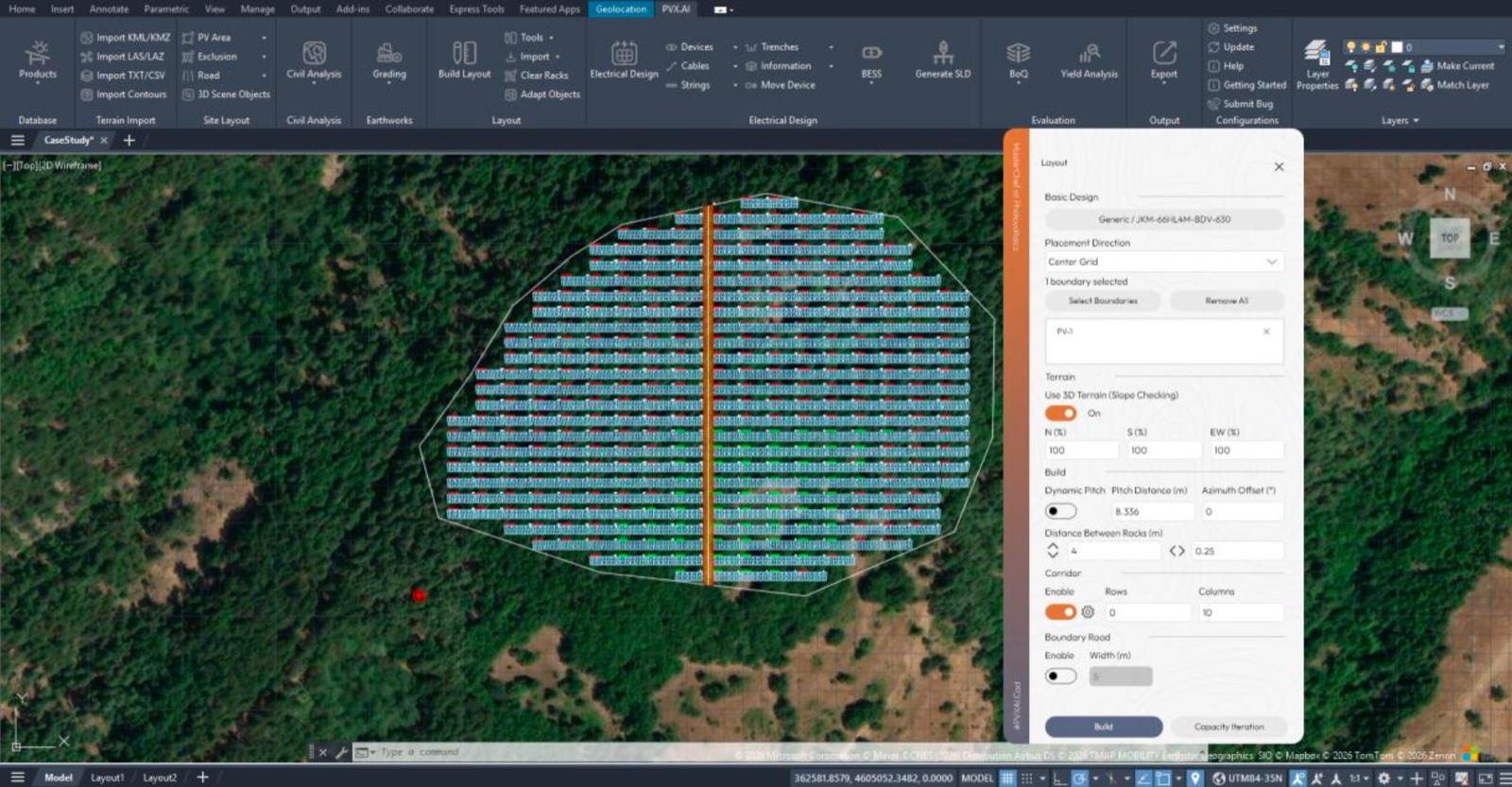
The nominal grid placed on the 3D terrain surface.
Coloring the racks by east-west slope makes the variation visible. The scale runs green to red with increasing gradient. This is the map of where the cosine effect will bite hardest.
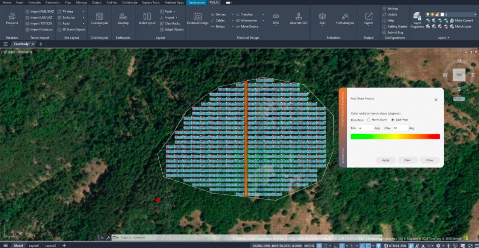
Rack-level slope analysis in the east-west direction.
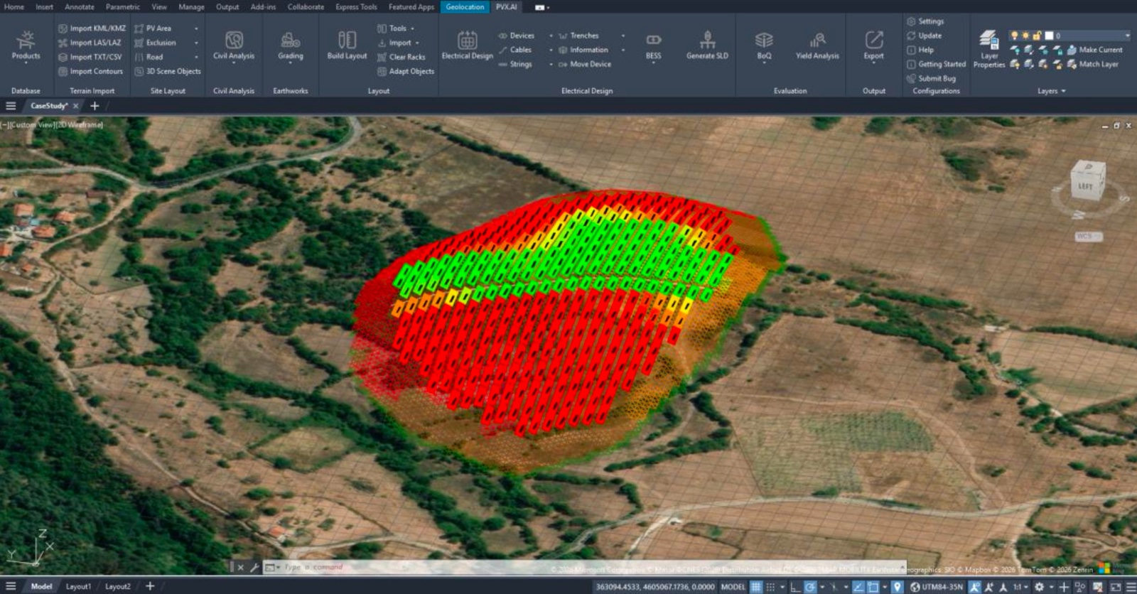
The same analysis in 3D perspective. The grid that looked uniform on the plan spreads unevenly across the real slope.
The cosine transformation
Here is the core of it. To verify how pile spacing behaves on the real surface, a reference line is drawn along the first vertical pile line and the parallelism of the pile rows is checked against it. The nominal 2.65 m bays measure 2.59 m and 2.58 m on the terrain.
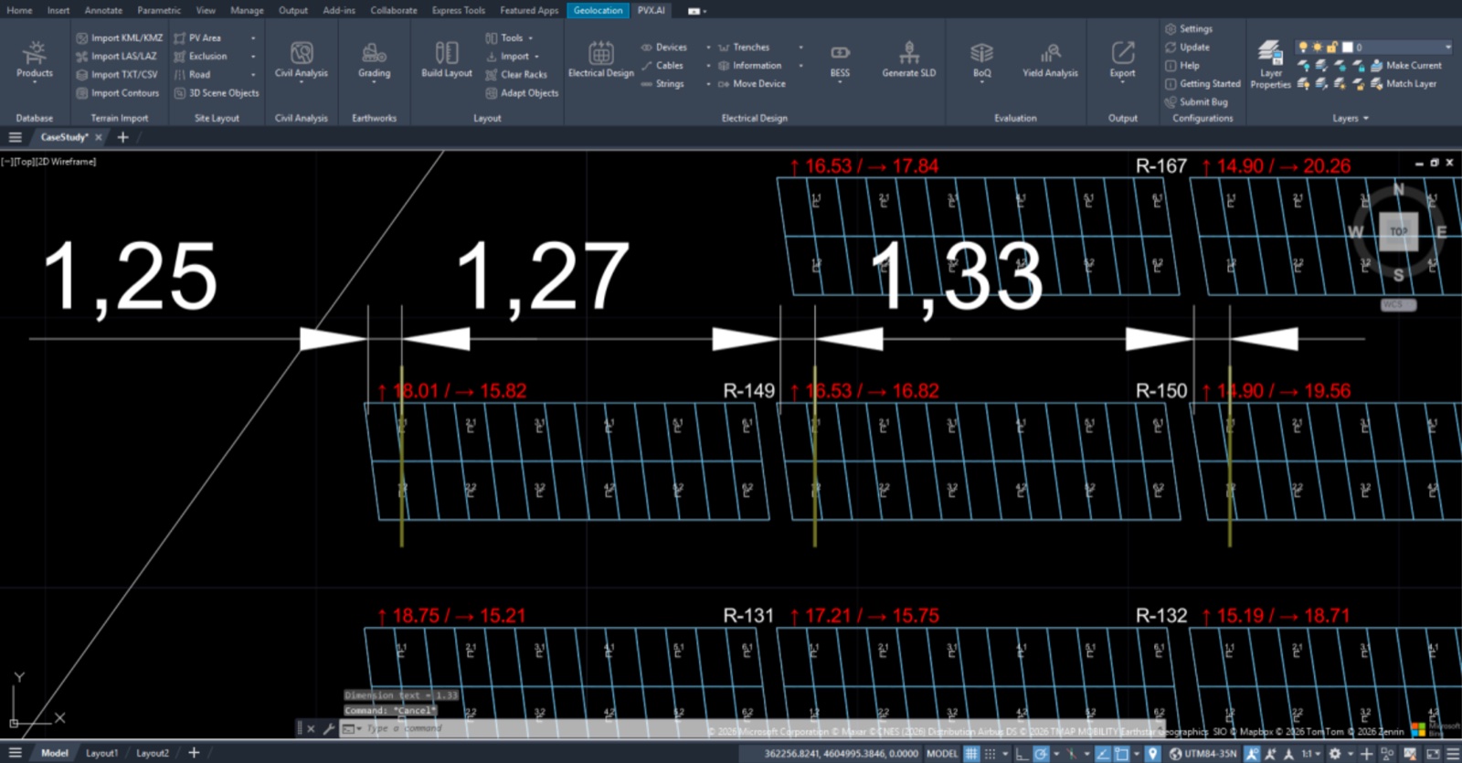
Parallelism check against a reference line. The plan says 2.65 m. The ground says less.
The mathematics is right-triangle trigonometry. The spacing measured along the rack plane is the hypotenuse. Its horizontal projection is the adjacent side. The angle between them is the terrain gradient θ along the pile row:
dhorizontal = drack × cos θ
Δz = drack × sin θ
θ = arccos(dhorizontal / drack) = arccos(2.58 / 2.65) ≈ 13.1°
In section view, the geometry looks like this:
The cosine projection in section. The 2.65 m held constant along the rack plane narrows to 2.58 m in the horizontal axis, while each pile base steps down 0.60 m. One slope angle produces both deviations at once.
The plan-view consequence: the rectangle becomes a parallelogram. The pile grid, defined orthogonal and equally spaced on the rack plane, shrinks by cos θ when projected to the ground. Where the slope direction is not perpendicular to the rack axis, the grid edges shear. Rows stay parallel to each other. What changes is the spacing and the angular form of the grid.
The same transformation in plan view. This is exactly why the racks in the site view above appear as parallelograms, not rectangles.
The cross-section front view confirms the relationship one-to-one on the real terrain. Nominal 2.65 m intervals measure 2.59 m and 2.58 m on the sloped ground. The ratio 2.58 / 2.65 ≈ 0.974 corresponds to roughly 13° of gradient, which matches the slope analysis values from the first step.
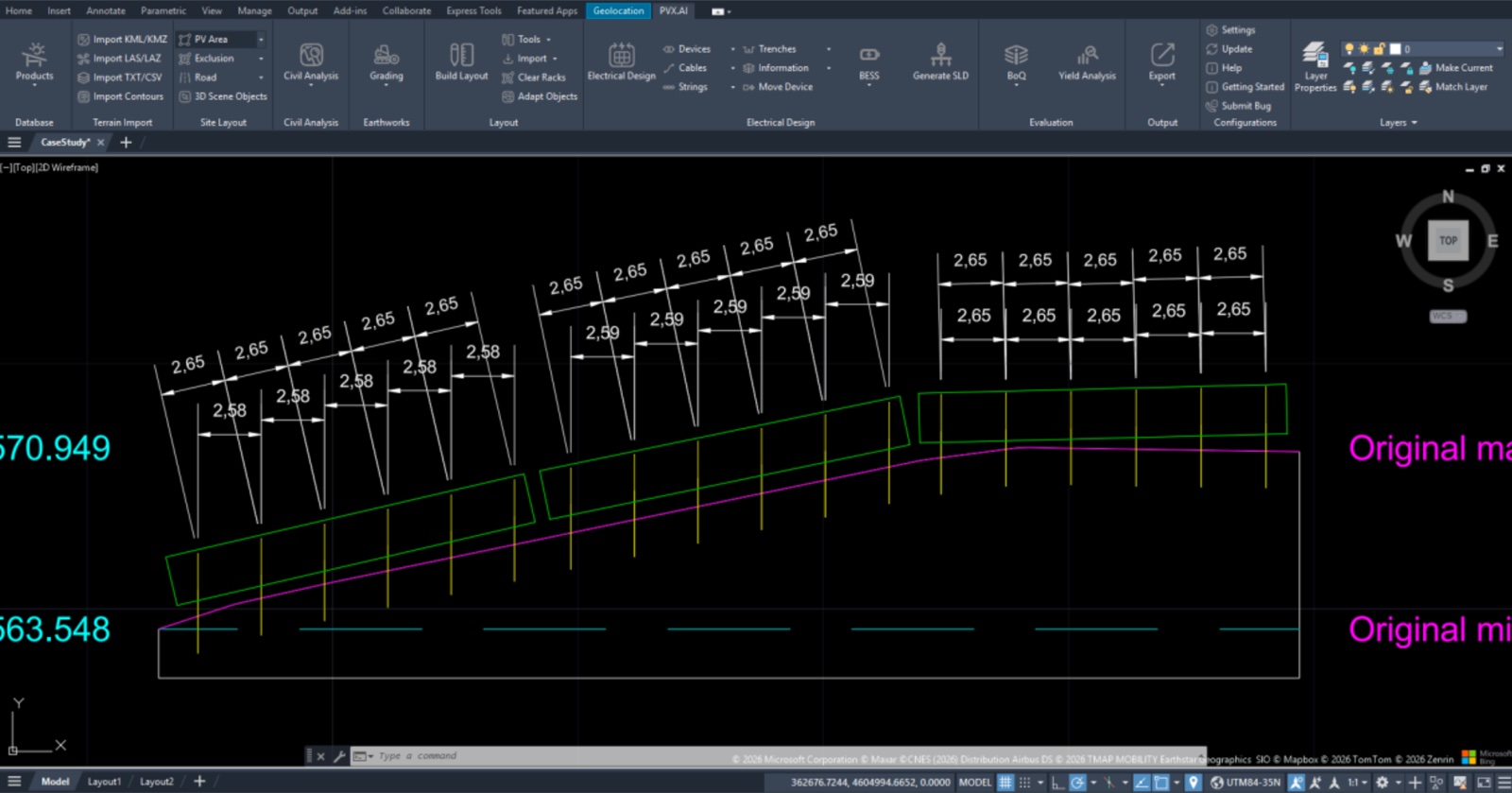
Cross-section verification: the nominal spacing, the narrowed horizontal projection, and the original terrain lines in one view.
The angle that matters is not the module tilt. The rack tilts modules at 25°. The spacing narrows by 13°. These are two different angles. Module tilt concerns the panel plane; the horizontal projection of pile spacing is governed by the gradient of the ground the piles are driven into, along the pile row. Confusing the two is one of the most common sources of coordinate errors in the field.
From geometry to coordinates: the pile schedule
The cosine transformation is not the deliverable. The deliverable is the pile schedule: recalculated positions exported as X, Y, and Z for every pile on the site. This is the information the field crew actually needs at staking, not a single one-dimensional interval from the plan, but verified three-dimensional coordinates for each pile, cross-checked against section views.
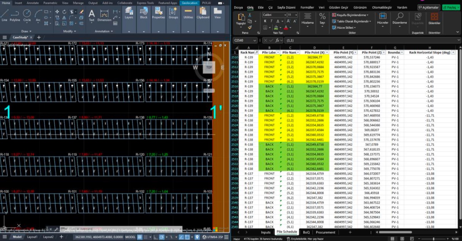
The exported pile schedule next to the drawing it was generated from. Every pile carries its own verified X-Y-Z position.
The Pile Point Z column exposes the second layer of the problem. Horizontal narrowing is only one dimension. Every pile also sits at a different elevation, so the schedule that leaves the design office has to carry the vertical answer too. The Rack Horizontal Slope column (−1.43°, −11.71°, −13.08° in this export) confirms what the slope map promised: the gradient changes from rack to rack, and with it the cosine factor. There is no single correction number for the site.
2D plan against 3D reality
Put the two worlds side by side. The plan view shows the ideal parallel grid, drawn without terrain. Clean, rectangular, evenly spaced. It is the world inside the designer’s head.
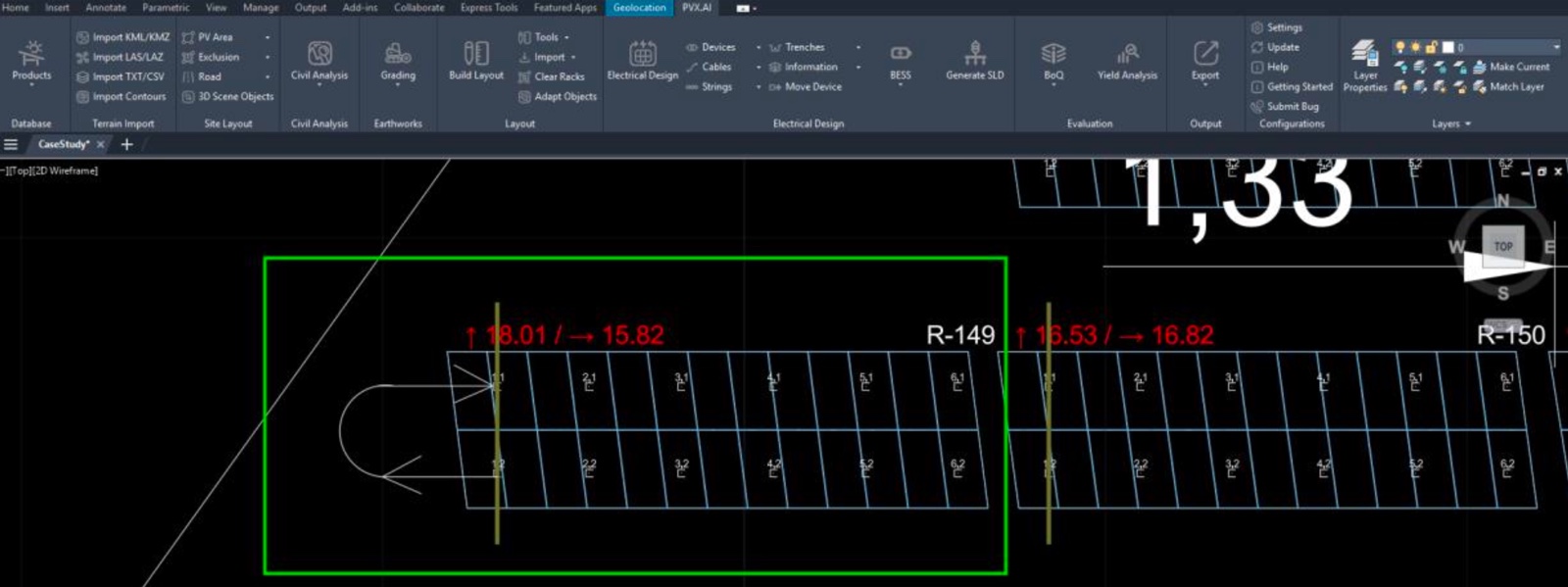
The naive parallel geometry in plan view.
The 3D view shows the same layout on the real site. Piles sit at different elevations, racks step down the gradient, and the grid shears with the topography.
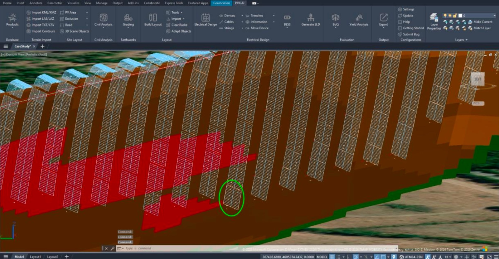
The same design on the real site. The difference between these two images is the gap the coordinate transformation closes.
What to take away
- Pile spacing that reads equal and uniform on the plan (2.65 m) narrows on sloped ground by the cosine projection (2.59 m, 2.58 m measured on this site).
- The operative angle is the terrain gradient along the pile row (θ ≈ 13.1° here), not the 25° module tilt.
- The same angle simultaneously produces an elevation step between piles: Δz = d × sin θ, about 0.60 m per bay on this site.
- Horizontal narrowing is half the story. Each pile sits at its own elevation, so the site needs full X-Y-Z coordinates for every pile.
- Cross-section views against the exported coordinates verify the transformation before anyone stakes anything.
The conclusion for practice: stake from verified coordinates, never from the paper dimension. On sloped sites the 2D plan alone will mislead; coordinates will not. PVX.Cad applies the cosine transformation automatically when the layout meets 3D terrain, and exports the pile schedule with section-view cross-checks built into the same workflow. The gap between the drawing and the site closes before the first pile goes in.
Related reading: the terrain-first methodology and what tracker architecture does to earthworks.