In a classical EPC workflow, the electrical design of a 30 MWp solar plant takes 3 to 4 weeks. The work spreads across AutoCAD for layout, PVsyst for production, and Excel for string sizing and cable schedules. Every handoff between tools loses data. On a recent pre-feasibility project in Türkiye (an anonymous 1,252 m site), PVX.Cad carried the entire flow, from 3D terrain model to per-string voltage drop, on one data model in 1 to 2 days.
This article walks through that design as engineering decisions, not button clicks. Behind every step is a constraint grounded in IEC or IEEE standards. The point is not that software designed the plant. The point is that the engineer spent the time on decisions instead of on data transfers.
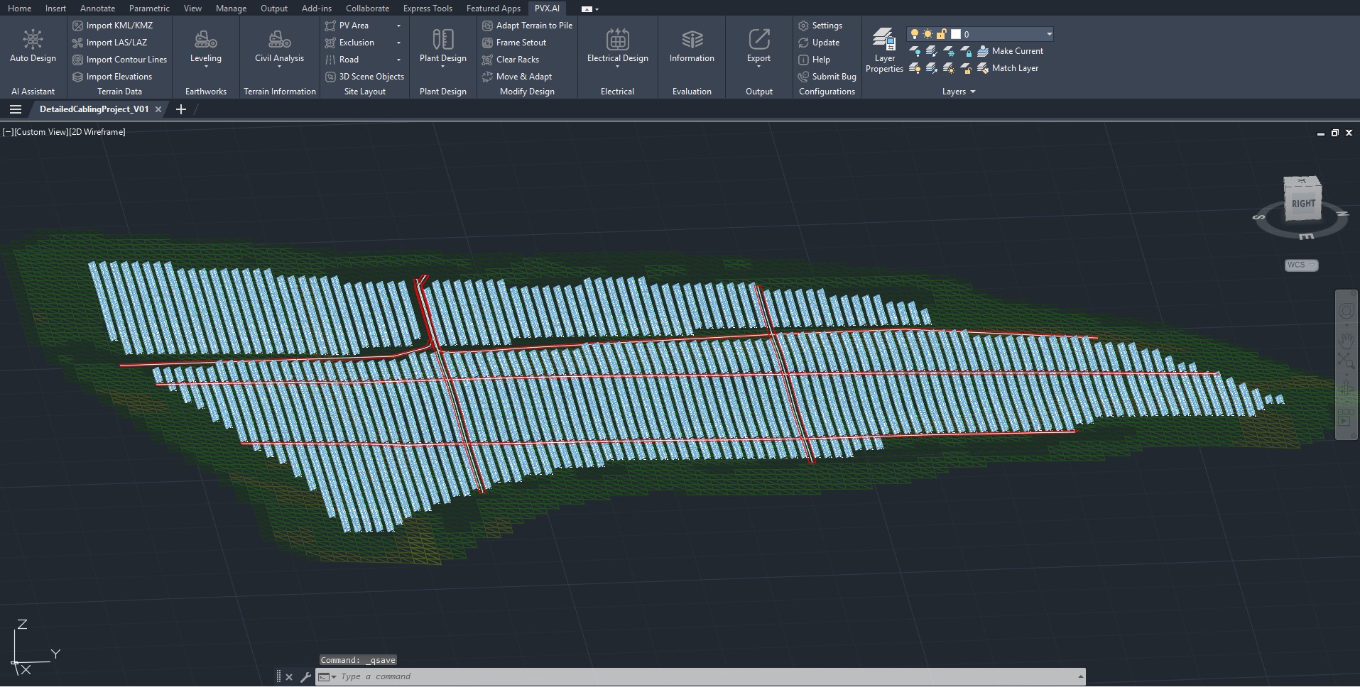 The 30 MWp array on east-facing terrain (70 degree aspect, 2.5 degree slope). DEM, exclusion zones, service roads, and rack placement all live on one 3D model.
The Plant
| Parameter | Value |
|---|---|
| Total DC capacity | 30,593 kWp |
| Total AC capacity | 29,750 kW |
| DC/AC ratio | 1.03 |
| Module | 540 Wp x 56,654 units |
| Inverter | Sungrow SG350-HX, 350 kW x 85 |
| Transformers | 5 x 4.65 MVA + 1 x 0.26 MVA aux |
| Strings | 2,165 (26 modules each) |
| Estimated net annual production | 50,318,693 kWh (50.3 GWh) |
| Performance ratio | 83.3% |
| Specific yield | 1,644.8 kWh/kWp/yr |
Standards referenced: IEC 62548-1, IEC 60364-7-712, IEC 60364-5-52, IEC 62930, IEC 61724-1, IEC 62446-1, IEEE 1547.
Site First: The Numbers That Drive Every Decision
The most expensive electrical mistakes are not made at the layout stage. They are made where the assumptions feeding the layout are wrong. Before designing anything, the site fingerprint sets the constraints:
- 1,252 m elevation, 2.5 degree slope, 70 degree (east) aspect. East-facing terrain means strong morning yield and a self-shading geometry that matters for row orientation.
- 117 snow days per year. Above the Türkiye average. This single number drives the string-sizing window, as shown below.
- 380 kV grid, 2.4 km away. Forces a two-stage step-up in the AC collection architecture.
PVX.Cad produces this read in one pass from DEM, GIS, and PVGIS data. The hours normally spent on data ingest collapse, and the designer goes straight to the decision phase.
String Sizing Is Set by the Coldest Morning
The heart of DC design is the string configuration. Too short and the string drops below the inverter MPPT window, losing power. Too long and it exceeds the inverter input voltage limit on a cold morning, risking equipment damage.
Module open-circuit voltage rises as temperature falls. So the design-limiting case is Voc at minimum temperature, not the summer peak. For a 26-module string at minus 10 degrees C:
- Voc(Tmin) = 1,414 V against the Sungrow SG350-HX’s 1,500 V limit. An 86 V margin.
- Vmpp at 70 degrees C cell temperature = 915 V, well above the 600 V MPPT lower limit.
The window is asymmetric: only 86 V to the upper bound, 315 V to the lower. That asymmetry is a direct consequence of the snow-day count, because cold sunny mornings drive the Voc spike. The string was set at 26 modules, near the center of the 17-to-27 window, deliberately leaving margin for harsher minus 15 degrees C radiative-cooling scenarios. PVX.Cad reads these characteristics from the module datasheet and warns on the fly, so the wrong string length is caught before it ships.
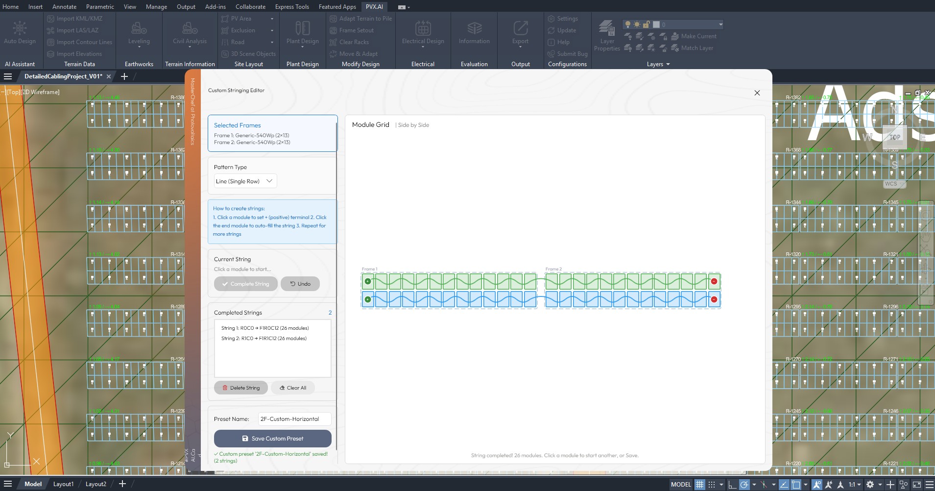 The Custom Stringing Editor. On 2-frame tables, two separate horizontal strings (one per frame) replace a single U-string, keeping mismatch inside the 2.0 percent envelope. Polarity is tracked automatically.
A second decision lived in the table geometry. On 2-frame tables, instead of a single U-string tying both frames into one MPPT chain, two separate horizontal strings were used, one per frame. The upper and lower frames see different shading, soiling, and thermal behavior. Splitting them keeps mismatch inside the 2.0% default envelope rather than the 2.5 to 3.0% a U-string typically carries.
Where You Put the Transformer Is a Cable-Cost Decision
The plant uses 85 inverters at 350 kW, distributed across 5 main transformers of 4.65 MVA each plus one 0.26 MVA auxiliary transformer for site loads (lighting, monitoring, SCADA). The DC/AC ratio of 1.03 is conservative on purpose: 117 snow days reduce winter production, so aggressive oversizing would only raise summer clipping without lifting the annual total.
The location of each transformer is the most important AC-loss decision in the plant. PVX.Cad computes a weighted load centroid from the coordinates of each transformer’s inverters and places the transformer there. This is the software realization of the classic p-median approach: minimize the sum of AC cable lengths from inverter outputs to transformer inputs. The hours of manual transformer-to-inverter mapping collapse to seconds, and automatic color coding gives each transformer zone a distinct color so the field crew can recognize at a glance which tables connect where.
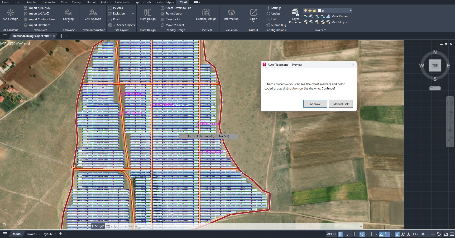 Five main transformers placed at the load centroid of each zone. Each transformer’s service radius is verifiable visually, and the AC cable length from inverters to transformer is minimized.
Trench Routing Follows the Service Roads
After DC is routed to each inverter, the AC collection topology begins. The trench backbone was aligned with the service roads, for three reasons grounded in practice and in IEC 60364-7-712:
- Service-road soil is already compacted, so trenching is easier and backfill quality is higher.
- Cable faults can be reached without further excavation.
- Cables under service roads have minimal mechanical exposure, so extra protection is minimized.
In the Cable Generation dialog, picking the system type (string, inverter, transformer) produces the entire site cable geometry in seconds, with each cable type carrying its own cross-section and trench class. Every cable segment auto-joins the nearest trench. That output is the direct data source for the bill of materials, with no manual segment-length tally in Excel.
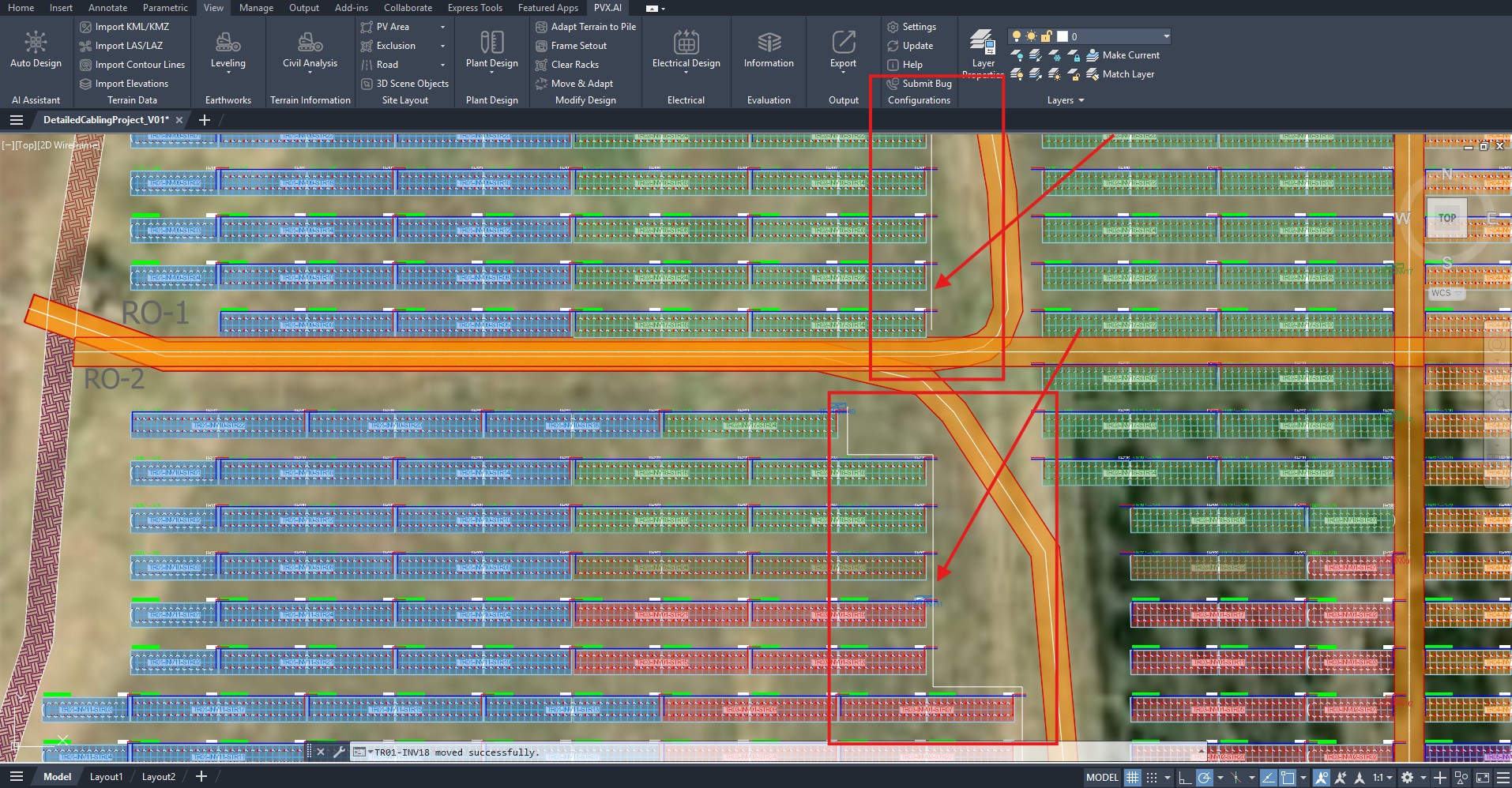 Trench backbones (orange) run directly under the service roads. DC string-end cables join the backbone from the row alleys; AC transformer outputs use it toward the grid exit.
Voltage Drop on All 2,165 Strings, Not One Average
This is where the design density shows. Classical workflows assume the average string is below the 2% IEC 62548 reference, because per-string calculation by hand is not feasible at utility scale. PVX.Cad traced every positive and negative DC cable in 3D and reported voltage drop per string across all 2,165 strings using real trench geometry. Values ranged from 1.39% to 1.87%.
One honest detail matters here. 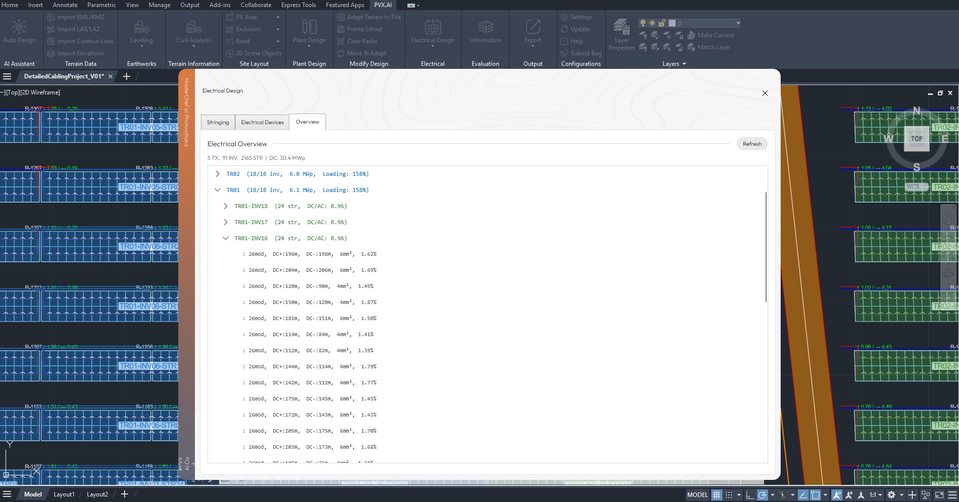 Per-string DC+ length, DC- length, cross-section, and voltage drop for every string under an inverter. Values range from 1.39 to 1.87 percent against the 1,500 V reference.
PVX.Cad reports voltage drop normalized to the system maximum operating voltage (1,500 V), which is a conservative reference for cable selection. Against the classical Vmpp reference, the worst-case string (a 204 m / 206 m loop) computes to 2.36%, just over the 2% IEC figure, where PVX reports 1.69% against 1,500 V. That is not a tool deficiency. It is a reference choice the engineer must interpret. The value of having the data on every string is precisely that this string surfaces as a layout-improvement signal: upgrade it to 6 mm cross-section, or shorten its inverter distance by about 30 m. Without per-string data, that string disappears into an average and ships as-is.
The practical takeaway: double-check both references on any string the report flags near the 2% limit. The data density to do that is the differentiator, not the convenience.
Classical EPC vs One Data Model
| Phase | Classical (CAD + Excel + post-process) | PVX.Cad |
|---|---|---|
| 3D terrain + layout | 3 to 5 days | under 30 min |
| String configuration | 5 to 7 days | 1 to 2 hours |
| Inverter-transformer balancing | 2 to 3 days | under 15 min |
| Trench + cable geometry | 3 to 5 days | under 1 hour |
| Per-string voltage drop | not done / estimated | automatic |
| Shading verification | 1 to 2 days | inline (3D viewer) |
| Total, sketch to bankable | 3 to 4 weeks | 1 to 2 days |
The value of the speed is not only fewer hours. It is iteration density. In a classical 3-week cycle, a designer tests one configuration. In the same period on one data model, a designer can test 10 or more: DC/AC ratio at 1.03 versus 1.20 versus 1.40, string length at 26 versus 24 versus 22 modules, trench plan A versus B.
What Does and Does Not Change for the Engineer
The IEC 62548 string-sizing derivation does not change. The IEEE 1547 inverter requirements do not change. The IEC 60364-5-52 derating assumptions do not change. Engineering judgment does not change.
What changes is the speed of applying that judgment, the visibility of a design’s side effects, and the ease of comparing alternatives. The engineer’s role grows, because time once spent drawing lines in AutoCAD is now spent deciding which design fits the site best. And when the plant is built, the output of the design, the string mapping, the voltage drop table, the trench backbone, the BOM, is in the field crew’s hands on day one. The most lasting product of a design is not a one-time layout file. It is a reliable reference for the operational life of the plant.