The Challenge
The electrical design of a utility-scale PV plant is usually framed as a layout problem followed by a stack of separate calculations. In a classical EPC workflow it spreads across AutoCAD for topography and layout, PVsyst for production, and Excel for string sizing and cable schedules. Each handoff loses data, and per-string verification is skipped because it is not feasible by hand.
This study walks the full electrical design of a 30 MWp plant (an anonymous pre-feasibility site in Türkiye at 1,252 m elevation) as a sequence of engineering decisions grounded in IEC and IEEE standards. PVX.Cad carried the entire flow, from 3D terrain model to per-string voltage drop, on a single data model.
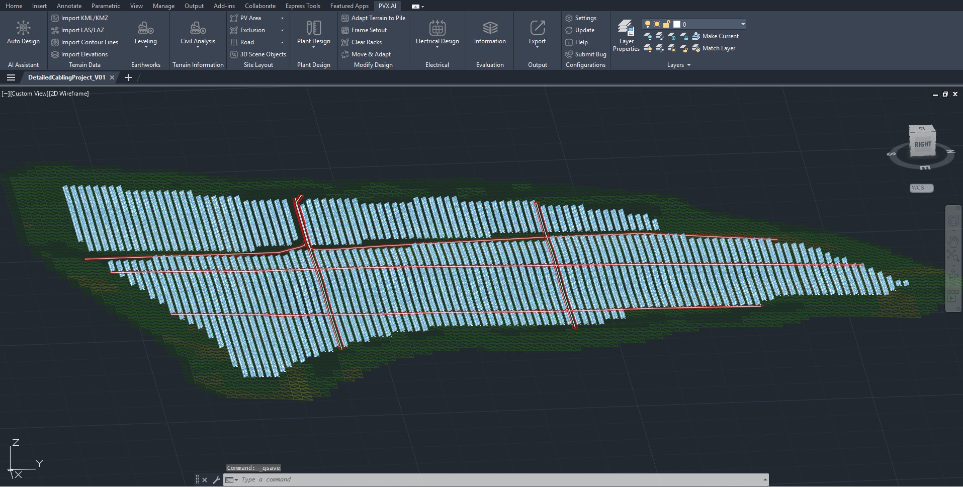 The 30 MWp array placed on the 3D terrain model. Service roads (red) divide the site into four maintenance zones that later become the AC trench backbone.
Plant Summary
| Parameter | Value | Reference |
|---|---|---|
| Total DC capacity | 30,593 kWp | PVX Prospect Report |
| Total AC capacity | 29,750 kW | After inverter config |
| DC/AC ratio | 1.03 | IEC 62548 conservative headroom |
| Module | 540 Wp x 56,654 units | Mono-PERC |
| Inverter | Sungrow SG350-HX, 350 kW x 85 | 1500 V DC system |
| Transformers | 5 x 4.65 MVA + 1 x 0.26 MVA aux | ~18 inverters each |
| Strings | 2,165 | 26 modules per string |
| Grid interconnection | 380 kV, 2.4 km | IEEE 1547 + TEDAS |
Site Fingerprint
The site sets the constraints before any design begins.
| Parameter | Value | Effect on design |
|---|---|---|
| Elevation | 1,252 m | Better cooling, harsh Tmin |
| Terrain slope | 2.5 degrees | Affects row pitch and self-shading |
| Aspect | 70 degrees (east) | Strong morning yield |
| GTI at optimal tilt | 1,974.8 kWh/m2/yr | DC production base |
| Snow days | 117 days/yr | Drives the Voc(Tmin) string limit |
| Nearest grid line | 380 kV, 2.4 km | Two-stage AC step-up |
PVX.Cad produces this read in one pass from DEM, GIS, and PVGIS data, so the time normally spent on data ingest goes to the decision phase instead.
String Sizing Window
Module open-circuit voltage rises as temperature falls, so the design-limiting case is the coldest morning, not the summer peak. For a 26-module string:
| Parameter | Value | Limit | Margin |
|---|---|---|---|
| Voc at minus 10 degrees C | 1,414 V | 1,500 V (inverter) | 86 V |
| Vmpp at 70 degrees C cell | 915 V | 600 V (MPPT lower) | 315 V |
| String Isc at STC | 13.6 A | 18 A (inverter input) | 32.5% |
The window is asymmetric: only 86 V of headroom to the upper bound versus 315 V to the lower. That asymmetry comes directly from the 117-snow-day climate. The string was set at 26 modules, near the center of the 17-to-27 window, leaving margin for harsher radiative-cooling scenarios. On 2-frame tables, two separate horizontal strings (one per frame) were used instead of a single U-string, keeping mismatch inside the 2.0% default envelope rather than the 2.5 to 3.0% a U-string typically carries.
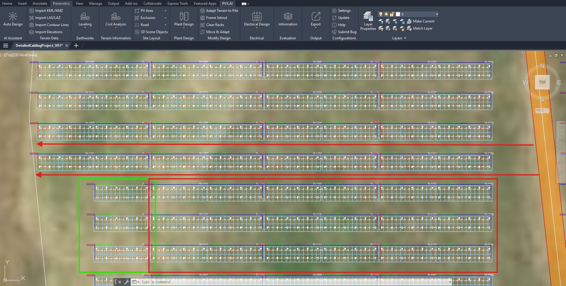 Auto-stringing complete. Red arrows show each string’s polarity output direction, which becomes the input for AC output verification and trench planning.
Transformer Placement
The plant uses 85 inverters at 350 kW across 5 main transformers (4.65 MVA each) plus one 0.26 MVA auxiliary transformer for site loads. The DC/AC ratio of 1.03 is deliberately conservative: 117 snow days cut winter production, so aggressive oversizing would only raise summer clipping without lifting the annual total.
Transformer location is the most important AC-loss decision in the plant. PVX.Cad computes a weighted load centroid from the coordinates of each transformer’s inverters and places the transformer at that point, a p-median approach that minimizes AC cable length from inverter outputs to transformer inputs. Automatic color coding then gives each transformer zone a distinct color, so the field crew can see at a glance which tables connect where.
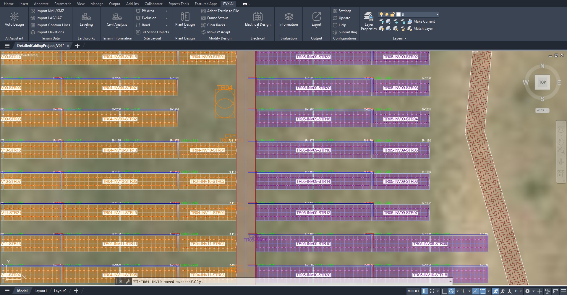 Five transformer zones in five colors. The field crew recognizes which tables connect to which transformer at a glance, reducing cabling-error risk at commissioning.
Trench Routing
The trench backbone was aligned with the service roads, for reasons grounded in IEC 60364-7-712: service-road soil is already compacted (easier trenching, better backfill), faults can be reached without further excavation, and mechanical exposure is minimal. Picking the system type in the Cable Generation dialog produced the entire site cable geometry in seconds, with each cable type carrying its own cross-section and trench class. Every segment auto-joined the nearest trench, which became the direct data source for the bill of materials.
Per-String Voltage Drop
PVX.Cad traced every positive and negative DC cable in 3D and reported voltage drop per string across all 2,165 strings, using real trench geometry rather than an average. Values ranged from 1.39% to 1.87%.
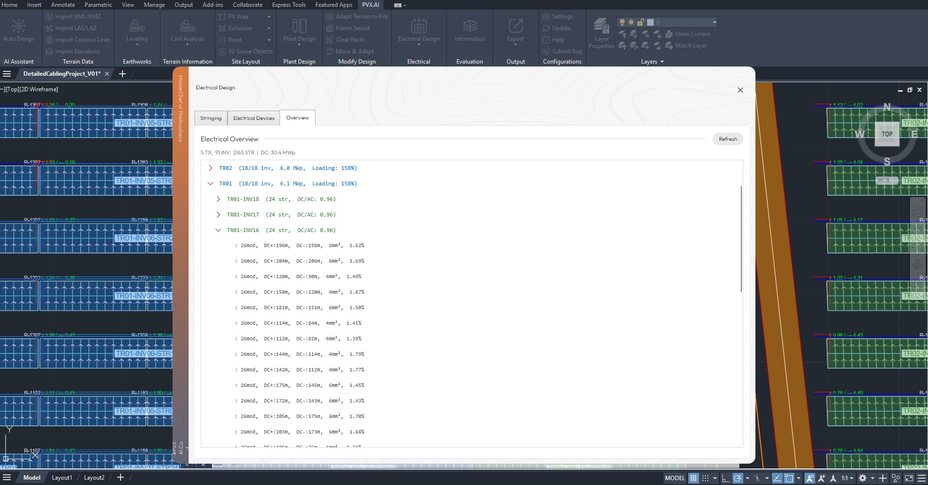 Each string’s DC+ length, DC- length, cross-section, and voltage drop. PVX.Cad delivers this for all 2,165 strings without a site visit.
PVX.Cad reports voltage drop normalized to the system maximum operating voltage (1,500 V), a conservative reference for cable selection. Against the classical Vmpp reference, the worst-case string (a 204 m / 206 m loop) computes to 2.36%, just over the 2% IEC 62548 figure, where PVX reports 1.69% against 1,500 V. Having the data on every string is what makes that string visible as a layout-improvement signal: upgrade it to 6 mm cross-section or shorten its inverter distance by about 30 m. Without per-string data, it would disappear into an average and ship as-is.
Production and Financial Outlook
| Parameter | Value |
|---|---|
| Annual net energy (AC) | 50,318,693 kWh (50.3 GWh) |
| Specific yield | 1,644.8 kWh/kWp |
| Performance ratio | 83.3% |
| Capacity factor (DC) | 18.8% |
| Total CapEx | 10,707,606 USD |
| Specific CapEx | 0.350 USD/Wp |
| Equity IRR (30 yr, indicative) | 33.8% |
| NPV (30 yr, indicative) | 38,734,469 USD |
Of the 16.7% total system loss, three components are directly under the electrical designer’s control: DC wiring (1.5%), AC wiring (0.8%), and shading (2.0%). With mismatch (2.0%), that is 6.3% of an ideal 60.4 GWh, or about 3.8 GWh per year, that the electrical design directly optimizes. The financial figures are indicative and require a bankable model with sensitivity analysis before financing, but a 33.8% indicative equity IRR places the project on a healthy preliminary footing.
Classical EPC vs One Data Model
| Phase | Classical workflow | PVX.Cad |
|---|---|---|
| 3D terrain + layout | 3 to 5 days | under 30 min |
| String configuration | 5 to 7 days | 1 to 2 hours |
| Inverter-transformer balancing | 2 to 3 days | under 15 min |
| Trench + cable geometry | 3 to 5 days | under 1 hour |
| Per-string voltage drop | not done / estimated | automatic |
| Shading verification | 1 to 2 days | inline |
| Total, sketch to bankable | 3 to 4 weeks | 1 to 2 days |
Key Findings
- Full electrical design ran in 1 to 2 days versus 3 to 4 weeks classically, on one data model with no manual handoffs between tools.
- String length was set by the coldest morning. Voc at minus 10 degrees C reached 1,414 V against the 1,500 V inverter limit, an 86 V margin driven by 117 snow days.
- Voltage drop was verified on all 2,165 strings (1.39 to 1.87%), not estimated from one average. The worst-case string surfaced as a fixable layout signal.
- Transformer placement used a load-centroid (p-median) method to minimize AC cable length, the single largest AC-loss lever in the plant.
- Two-frame horizontal stringing kept mismatch inside the 2.0% envelope, worth roughly 250 to 500 MWh per year.
- Iteration density, not just speed, is the gain. The same 3-week classical cycle that yields one configuration yields 10 or more on a single data model.