A solar layout can be complete in every drawing sense and still be wrong about the water. The rows are placed, the roads are cut, the trenches are routed. Then the first heavy storm finds the low line across the site, and it runs where it always ran: along a trench, under a row, across a road. Washouts along the cable route, standing water under the trackers, a transformer pad on ground that drains toward it. The O&M team inherits all of it for the life of the plant.
By the time you see it on site, the fix is earthworks, not edits. Hydrology Analysis and Erosion Controls in PVX.Cad exist to put the same information in the drawing weeks earlier, where it costs a layer toggle to look at and a layout edit to act on.
This post walks through one run on a real layout: a 27.67 MWp terrain-following tracker site in Spain, 766 racks and 42,896 modules on a 49.15 ha PV area. Every number below is read off the screen.
One thing to say up front: neither analysis moves anything. PVX draws the water and the soil loss in your DWG. Where the racks and the transformer go stays your decision.
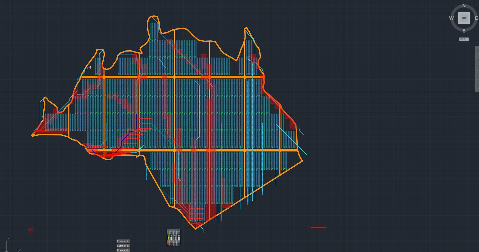
The layout after the hydrology run. Channels in cyan, roads in orange, and the ground a transformer should avoid in red, on its own layer.
Two questions the terrain answers
The two analyses answer two different questions about the same surface.
Where does the water go? Hydrology Analysis reads the imported terrain and draws the natural drainage network: the channels, the direction of flow along them, the subcatchments that feed them, and the points where water leaves the site. It also grades the ground for equipment placement.
What does it take with it? Erosion Controls computes soil loss across the site for a design storm, maps it in three bands, and places sized structures where the model says they are warranted: check dams in the channel reaches, diversion swales on the upslope edge of high-erosion ground, silt fences where sheet flow reaches the boundary, sediment basins at the outlets.
Both run as cloud jobs from inside AutoCAD. Both draw their results as native AutoCAD entities on their own layers, so they sit in the same DWG as the racks and the roads and turn on and off like any other layer.
Hydrology Analysis: where the water goes
The command sits on the Civil Analysis tab, in the Analysis panel, next to Soil Compaction and Erosion Controls. The dialog has no inputs. It explains what will be drawn and asks you to pick the PV area.
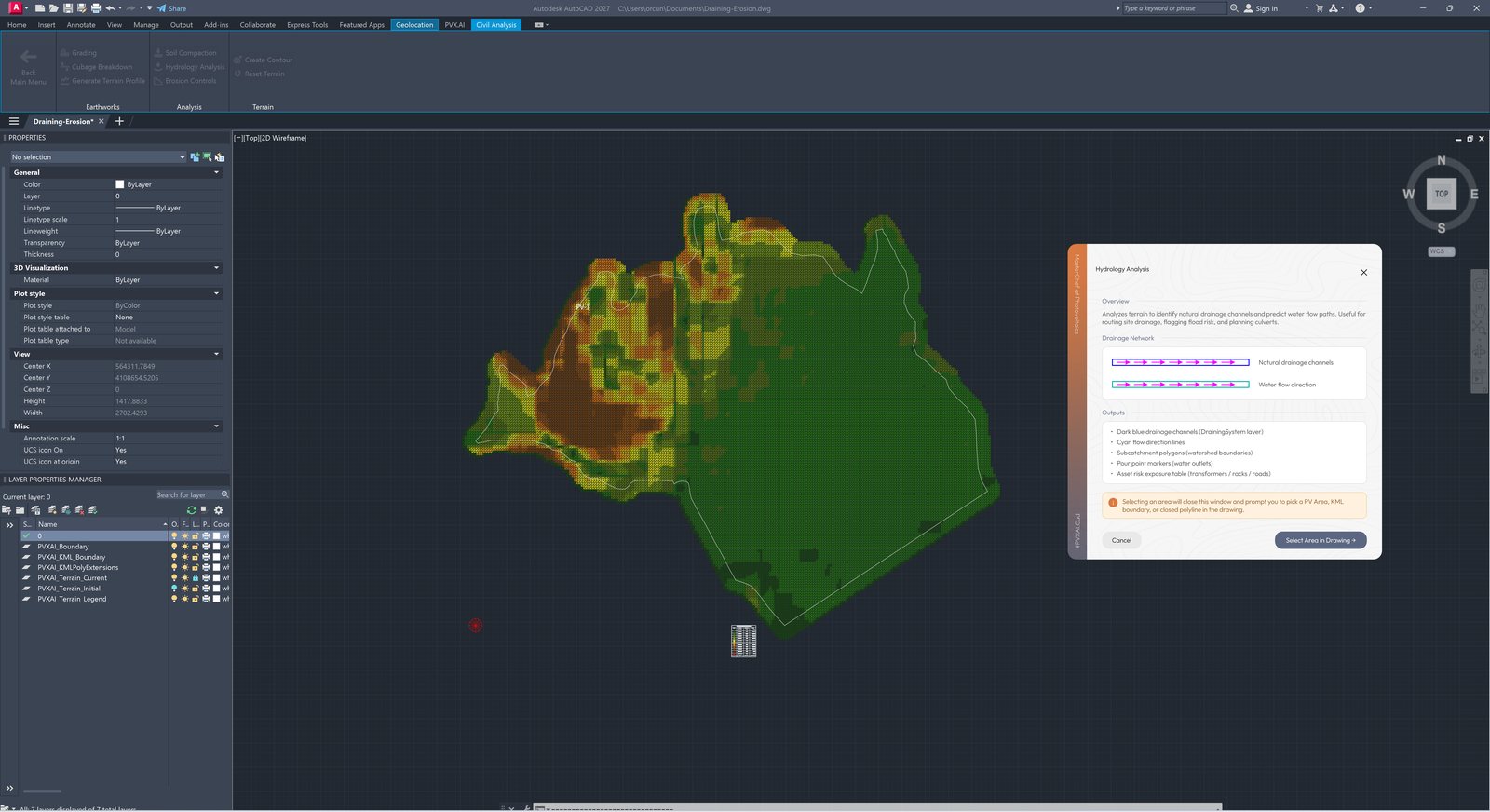
The dialog before the run. The terrain behind it is coloured by slope; the PV area boundary is PV-1.
Select the PV area polyline and the job runs: collecting drainage data, creating the network, drawing it. The command line reports what came back.
| Drawn on the site | Count |
|---|---|
| Drainage lines | 62 |
| Flow direction arrows | 2,263 |
| Subcatchment boundaries | 18 |
| Pour points | 21 |
| Placement suitability | 95.9% suitable, 0.0% caution, 4.1% avoid |
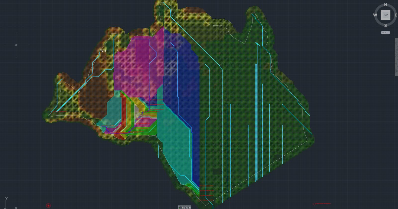
The drainage network over the terrain, before the racks are placed. Natural channels are dark blue, synthetic connections turquoise, and each subcatchment gets its own hatch colour.
The channels are 1 m wide polylines on the PVXAI_DrainingSystem layer, so they are a real width on the plan, not a hairline. The flow arrows sit directly on them. The subcatchments are transparent hatches on their own layer, one colour per catchment, so you can read which part of the site feeds which channel.
The pour points are the useful part for the boundary. Each one is a red circle with a label: its name, its type, and the contributing area in hectares.
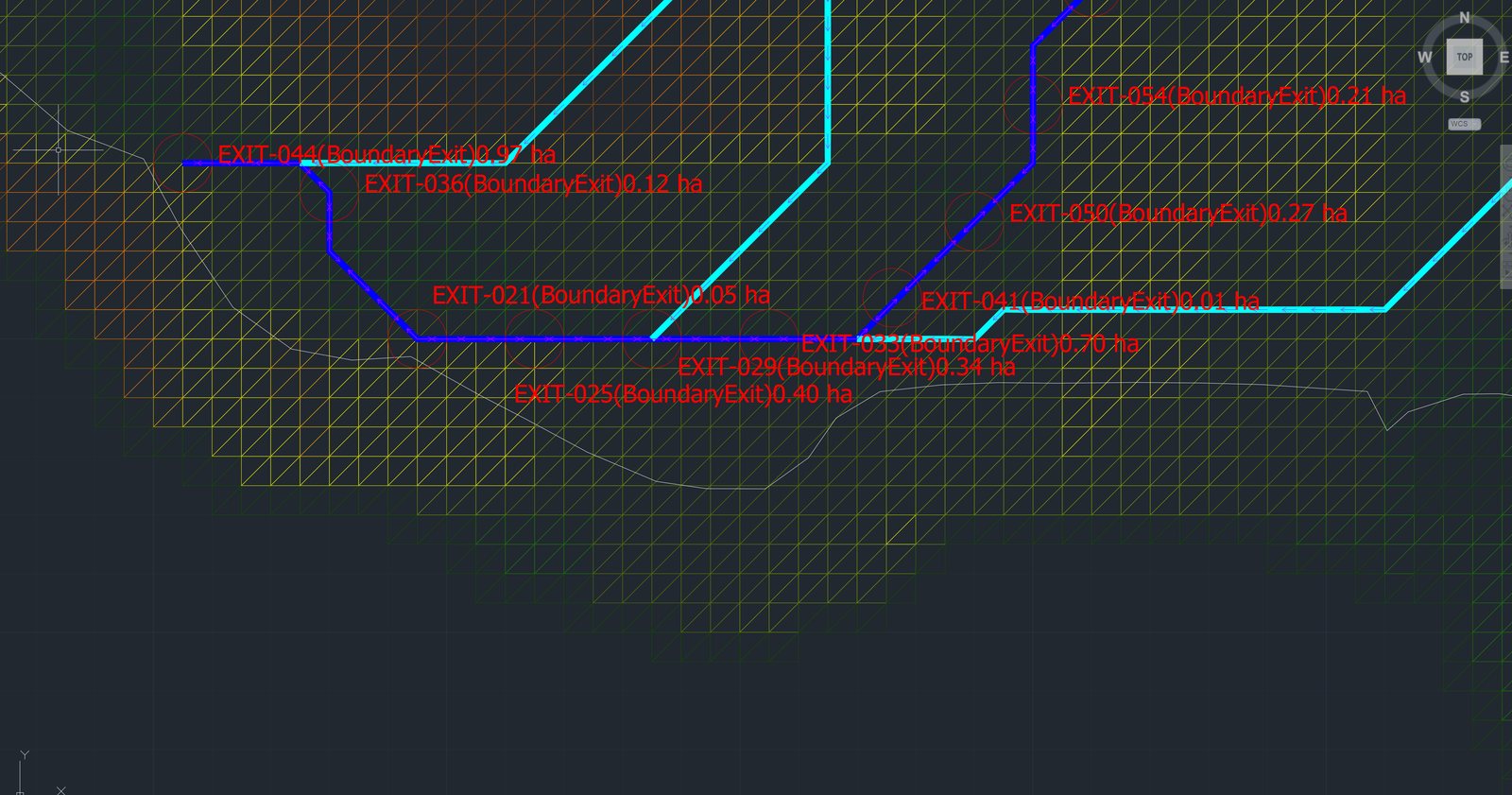
Where the water leaves the site. EXIT-044 carries 0.97 ha, EXIT-033 0.70 ha, EXIT-025 0.40 ha. Twenty-one outlets in total.
That is the list you hand the civil engineer for the perimeter: 21 places where water crosses the fence line, each with the area behind it.
Where the transformer can stand
The same run colours the ground for equipment placement. Green is suitable, yellow is caution, red is avoid, each on its own layer (PVXAI_DrainingSystem_Suitability_Suitable, _Caution, _Avoid), and the command line prints the split. On this site: 95.9% suitable, 0.0% caution, 4.1% avoid.
The red follows the channels. In the plan view at the top of this post, the avoid zones run along the cyan lines through the rows and along the southern edge where the channels converge. Turn the racks off and the picture is the same one a civil engineer would draw by hand from the contours, except it is already in the DWG.
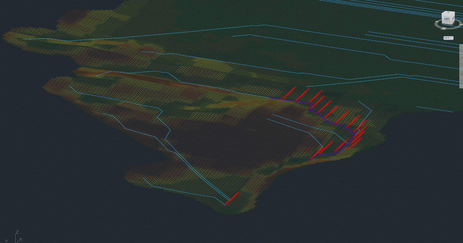
The same avoid zones in 3D. They sit in the channel corridors where the terrain concentrates the flow.
When transformers are already in the drawing, the run also draws a drainage risk table beside the site, one row per transformer: its catchment, the upstream area in hectares, the local accumulation, the distance to the nearest channel and to the outlet, a low, medium or high rating and an action. The rows are coloured green, yellow and red like the zones. This drawing had no transformers placed yet, so no table was drawn. Place them on green ground and the table confirms it.
Channels under the rows
The picture that matters for the layout is the one where the water crosses the racks.
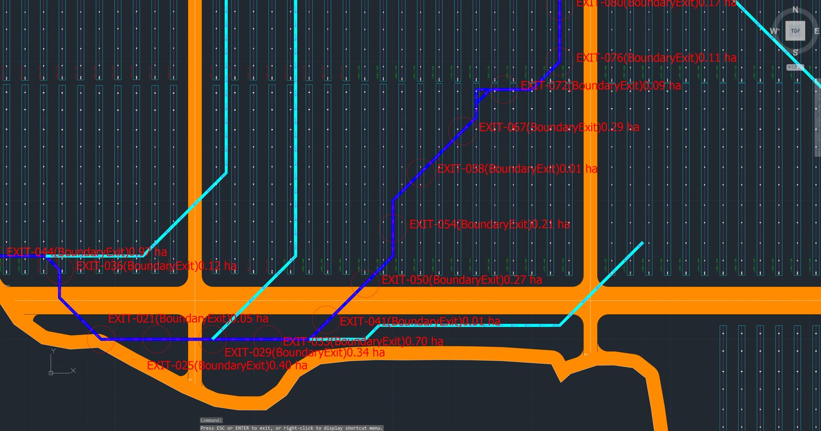
A channel crossing under the tracker rows and running along the road. The rows stay where they are; the drawing shows you what runs beneath them.
Terrain-following trackers can stand over a channel. Their piles are in the ground either way, and the analysis does not lift or move them. What changes is what you route through that corridor. A DC trench dug along a channel becomes the channel. A road that crosses it without a culvert becomes a dam. A transformer pad in the red becomes the low point everything drains to.
None of that is decided by the software. The channel is on its layer, the racks are on theirs, and the decision to keep the trench on the other side of the row is yours. What you no longer have to do is guess where the water is.
Erosion Controls: what the water takes with it
The second command sits next to the first. Its dialog does take inputs.
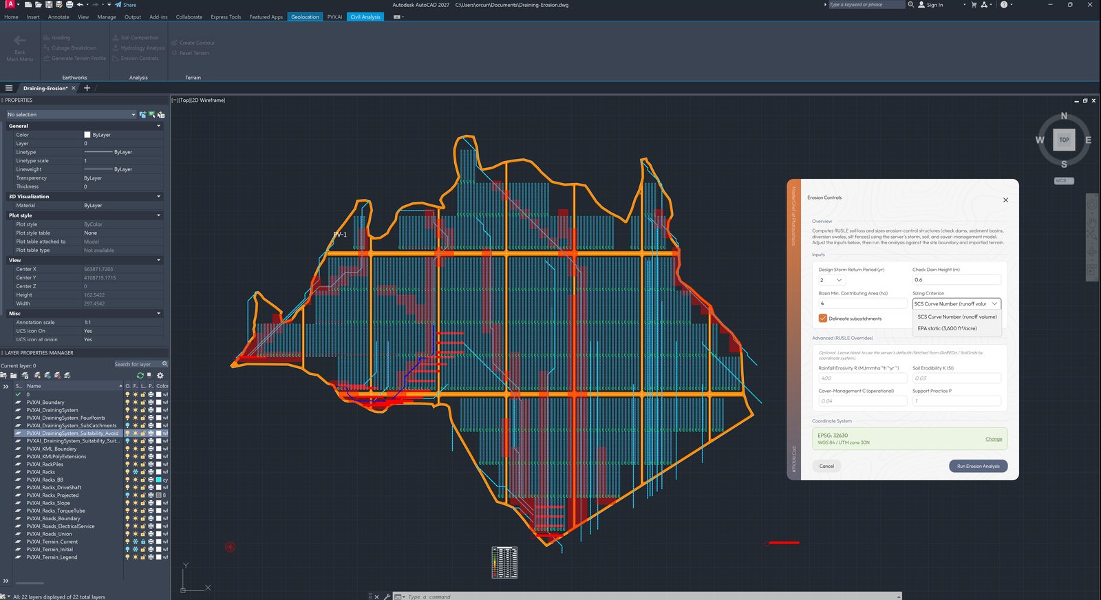
The dialog with its defaults. The coordinate system is EPSG 32630, WGS 84 / UTM zone 30N.
| Input | Value used |
|---|---|
| Design storm return period | 2 years (options: 2, 5, 10, 25, 50, 100) |
| Check dam height | 0.6 m |
| Basin minimum contributing area | 4.0 ha |
| Sizing criterion | SCS Curve Number (runoff volume); EPA static 3,600 ft³/acre is the alternative |
| Delineate subcatchments | On |
| RUSLE overrides (R, K, C, P) | Blank, so the server fetches defaults for the site |
The RUSLE factors come from global datasets for the site location: rainfall erosivity R from JRC GloREDa, soil erodibility K and the hydrologic soil group from ISRIC SoilGrids, cover management C from ESA WorldCover. If you have measured values, type them in and they replace the defaults. The site boundary is taken from the PVXAI_Boundary layer, and the drawing needs a coordinate system set, because the datasets are looked up by location.
Run Erosion Analysis, and the site comes back in three bands.
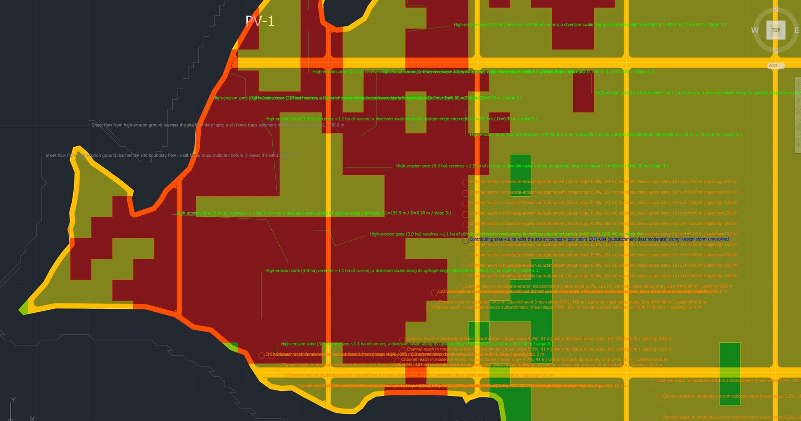
Part of the soil-loss map on the PVXAI_Erosion_Risk layer, zoomed to the steep western end of the site. Red is over 50 t/ha/yr, yellow 10 to 50, green under 10. The labels belong to the structures placed on it.
The view above is a zoomed part of the site, its steepest ground, and it is mostly red because slope is the largest factor in RUSLE: the same rain takes more soil off a 10% grade than off a 3% one. Across the whole PV area the bands mix, and the red concentrates where the terrain is steep and where the channels run. The structures are placed against that map.
The structures, with their reasons
Every structure the model places carries a label with two lines: why it is there, and what size it is. Reading a few of them off the drawing:
- Check dams. “Channel reach in moderate-erosion subcatchment (mean slope 6.0%, 161 m) warrants check dams every 10 m. H=0.60 m / spacing=10.0 m.” On a shallower reach (4.9%, 133 m) the spacing opens to 12.2 m.
- Diversion swales. “High-erosion zone (3.0 ha) receives ~1.1 ha of run-on; a diversion swale along its upslope edge intercepts it. L=134.9 m / D=0.30 m / slope 3:1.” Others read L=73.3 m, 45.0 m, 25.0 m and 20.0 m, same depth, same side slopes.
- Silt fences. “Sheet flow from high-erosion ground reaches the site boundary here; a silt fence traps sediment before it leaves the site. L=138.6 m.”
- Sediment basins. “Contributing area 4.8 ha exits the site at boundary pour point EXIT-084 (subcatchment class moderate).” The basin sits at the outlet the hydrology run found.
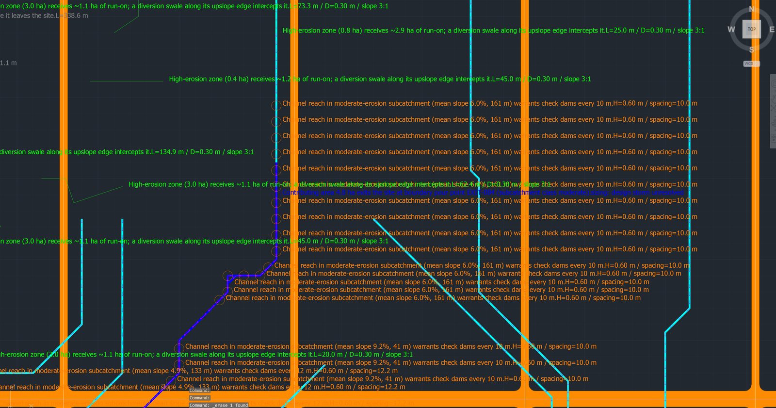
Check dams every 10 m along a channel reach, each with its height and spacing in the label. The swale and silt fence labels sit on the ground they protect.
Beside the site, the run draws the bill of quantities.
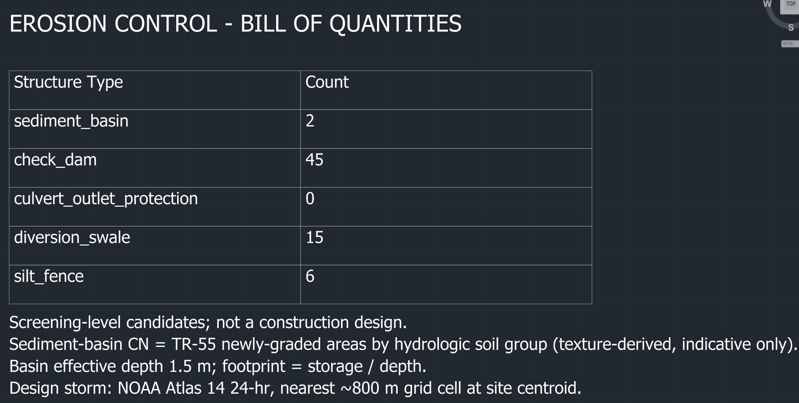
The bill of quantities as drawn, footnotes included.
| Structure | Count |
|---|---|
| Check dams | 45 |
| Diversion swales | 15 |
| Silt fences | 6 |
| Sediment basins | 2 |
| Culvert outlet protection | 0 |
The footnotes under the table are part of the deliverable. The first one reads: “Screening-level candidates; not a construction design.” The others state the assumptions: the basin curve number follows TR-55 newly graded areas by hydrologic soil group, the basin effective depth is 1.5 m with footprint equal to storage over depth, and the design storm is a NOAA Atlas 14 24-hour depth at the site centroid.
That last footnote explains the one line on this drawing that reads “sizing: design storm unresolved”, on both basins. NOAA Atlas 14 covers the United States. This site is in Spain, so the model placed each basin at its outlet and reported its contributing area, and left the volume to be sized with the local rainfall data. On a US site the same run returns storage and footprint on the basin label. The check dams, swales and silt fences are sized either way, because their dimensions follow the slope, the reach length and the run-on area, not the storm depth.
Culvert outlet protection is zero here because no culverts were sized in this run. Where a road crosses a channel, PVX.Cad sizes the culvert from a design rainfall you enter in the Grading dialog, and the erosion run then protects its outlet. On this site that step was not run.
What this is, and what it is not
It is a screening and sizing pass on the terrain you already imported, drawn into the design you already have. RUSLE gives annual soil loss, the SCS method gives runoff volume, and the structures are candidates with first dimensions and stated reasons.
It is not a hydraulic model, and it is not the permit drainage design. The bill of quantities says so in its first footnote. What it gives the civil engineer is the location of every channel and outlet, the ground to keep the transformer off, the reaches that need check dams and at what spacing, the run-on that needs a swale and how long, and the perimeter that needs a fence, all in the DWG the layout lives in, before anyone grades.
Everything stays on layers you can list: PVXAI_DrainingSystem, _SubCatchments, _PourPoints, the three _Suitability_* layers, PVXAI_Erosion_Risk, _Zones, _CheckDams, _Swales, _SiltFence, _Basins, _Culverts and _BOQ. Turn them off for the layout drawing, on for the civil review.
Run it on your own site
Both analyses need a terrain and a boundary, nothing else. Import the terrain, draw or convert the PV area, and run Hydrology Analysis from the Civil Analysis tab. Set a coordinate system and run Erosion Controls from the same panel.
- Start a free trial of PVX.Cad and run both on your own terrain, inside your own AutoCAD. PVX.Cad is also listed on the Autodesk App Store.
- Book a demo and bring a DWG. We run the hydrology and erosion passes live on your site.
- Read more about the terrain analysis tools, the three ways to grade, and the pre-design site assessment report that carries the same analyses.